Text analysis 
 📃Dr. Çetinkaya-Rundel1 / 59

Announcements

This week's recap email will have instructions on checking/confirming your marks so far on Learn
Don't forget to turn in peer feedback for projects (for your team and other teams) by 17:00 today
HW 10 due Friday: You can use lower number of bootstrap samples, e.g. 1000.
OQ 10 due Friday: Last item due!
Making your project repo public (optional)

2 / 59

Piazza awards!

Congratulations to the winners!

3 / 59

Stickers!

Watch your email to find out when they'll be ready to pick up at my office. You can also stop by next term!

4 / 59

Save the date!

ASA DataFest @ EDI

Weekend-long data analysis hackathon, focusing on exploration, visualization, modeling, and insights

March 13 - 15, 2020
Bayes Centre
bit.ly/datafest-edi
Sign-up opens soon!

5 / 59

Tidytext analysis

6 / 59

Packages

In addition to tidyverse we will be using four other packages today

library(tidytext)
library(genius)
library(wordcloud)
library(DT)

7 / 59

Tidytext

Using tidy data principles can make many text mining tasks easier, more effective, and consistent with tools already in wide use.
Learn more at https://www.tidytextmining.com/.

8 / 59

What is tidy text?

text <- c("Take me out tonight",
          "Where there's music and there's people",
          "And they're young and alive",
          "Driving in your car",
          "I never never want to go home",
          "Because I haven't got one",
          "Anymore")
text

## [1] "Take me out tonight"                   
## [2] "Where there's music and there's people"
## [3] "And they're young and alive"           
## [4] "Driving in your car"                   
## [5] "I never never want to go home"         
## [6] "Because I haven't got one"             
## [7] "Anymore"

9 / 59

What is tidy text?

text_df <- tibble(line = 1:7, text = text)
text_df

## # A tibble: 7 x 2
##    line text                                  
##   <int> <chr>                                 
## 1     1 Take me out tonight                   
## 2     2 Where there's music and there's people
## 3     3 And they're young and alive           
## 4     4 Driving in your car                   
## 5     5 I never never want to go home         
## 6     6 Because I haven't got one             
## 7     7 Anymore

10 / 59

What is tidy text?

text_df %>%
  unnest_tokens(word, text)

## # A tibble: 32 x 2
##     line word   
##    <int> <chr>  
##  1     1 take   
##  2     1 me     
##  3     1 out    
##  4     1 tonight
##  5     2 where  
##  6     2 there's
##  7     2 music  
##  8     2 and    
##  9     2 there's
## 10     2 people 
## # … with 22 more rows

11 / 59

What are you listening to?

12 / 59

From the "Getting to know you" survey

"What are your 3 - 5 most favorite songs right now?"

listening <- read_csv("data/listening.csv")
listening

## # A tibble: 104 x 1
##    songs                                                                   
##    <chr>                                                                   
##  1 Gamma Knife - King Gizzard and the Lizard Wizard; Self Immolate - King …
##  2 I dont listen to much music                                             
##  3 Mess by Ed Sheeran, Take me back to london by Ed Sheeran and Sounds of …
##  4 Hate Me (Sometimes) - Stand Atlantic; Edge of Seventeen - Stevie Nicks;…
##  5 whistle, gogobebe, sassy me                                             
##  6 Shofukan, Think twice, Padiddle                                         
##  7 Groundislava - Feel the Heat (Indecorum Remix), Nominal - Everyday Ever…
##  8 Loving you - passion the musical, Senorita - Shawn Mendes and Camilla C…
##  9 lay it down slow - spiritualised, dead boys - Sam Fender, figure it out…
## 10 Don't Stop Me Now (Queen), Finale (Toby Fox), Machine in the Walls (Mud…
## # … with 94 more rows

13 / 59

Looking for commonalities

listening %>%
  unnest_tokens(word, songs) %>%
  count(word, sort = TRUE)

## # A tibble: 786 x 2
##    word      n
##    <chr> <int>
##  1 the      56
##  2 by       23
##  3 to       20
##  4 and      19
##  5 i        19
##  6 you      15
##  7 of       13
##  8 a        11
##  9 in       11
## 10 me       10
## # … with 776 more rows

14 / 59

Stop words

In computing, stop words are words which are filtered out before or after processing of natural language data (text).
They usually refer to the most common words in a language, but there is not a single list of stop words used by all natural language processing tools.

15 / 59

English stop words

get_stopwords()

## # A tibble: 175 x 2
##    word      lexicon 
##    <chr>     <chr>   
##  1 i         snowball
##  2 me        snowball
##  3 my        snowball
##  4 myself    snowball
##  5 we        snowball
##  6 our       snowball
##  7 ours      snowball
##  8 ourselves snowball
##  9 you       snowball
## 10 your      snowball
## # … with 165 more rows

16 / 59

Spanish stop words

get_stopwords(language = "es")

## # A tibble: 308 x 2
##    word  lexicon 
##    <chr> <chr>   
##  1 de    snowball
##  2 la    snowball
##  3 que   snowball
##  4 el    snowball
##  5 en    snowball
##  6 y     snowball
##  7 a     snowball
##  8 los   snowball
##  9 del   snowball
## 10 se    snowball
## # … with 298 more rows

17 / 59

Various lexicons

See ?get_stopwords for more info.

get_stopwords(source = "smart")

## # A tibble: 571 x 2
##    word        lexicon
##    <chr>       <chr>  
##  1 a           smart  
##  2 a's         smart  
##  3 able        smart  
##  4 about       smart  
##  5 above       smart  
##  6 according   smart  
##  7 accordingly smart  
##  8 across      smart  
##  9 actually    smart  
## 10 after       smart  
## # … with 561 more rows

18 / 59

Dr. Mine Çetinkaya-Rundel -
introds.org


Back to: Looking for commonalitieslistening %>%
  unnest_tokens(word, songs) %>%
  anti_join(stop_words) %>%
  filter(!(word %in% c("1", "2", "3", "4", "5"))) %>%
  count(word, sort = TRUE)

## Joining, by = "word"
## # A tibble: 640 x 2
##    word        n
##    <chr>   <int>
##  1 ed          7
##  2 queen       7
##  3 sheeran     7
##  4 love        6
##  5 bad         5
##  6 time        5
##  7 1975        4
##  8 dog         4
##  9 king        4
## 10 life        4
## # … with 630 more rows
19 / 59

Dr. Mine Çetinkaya-Rundel -
introds.org


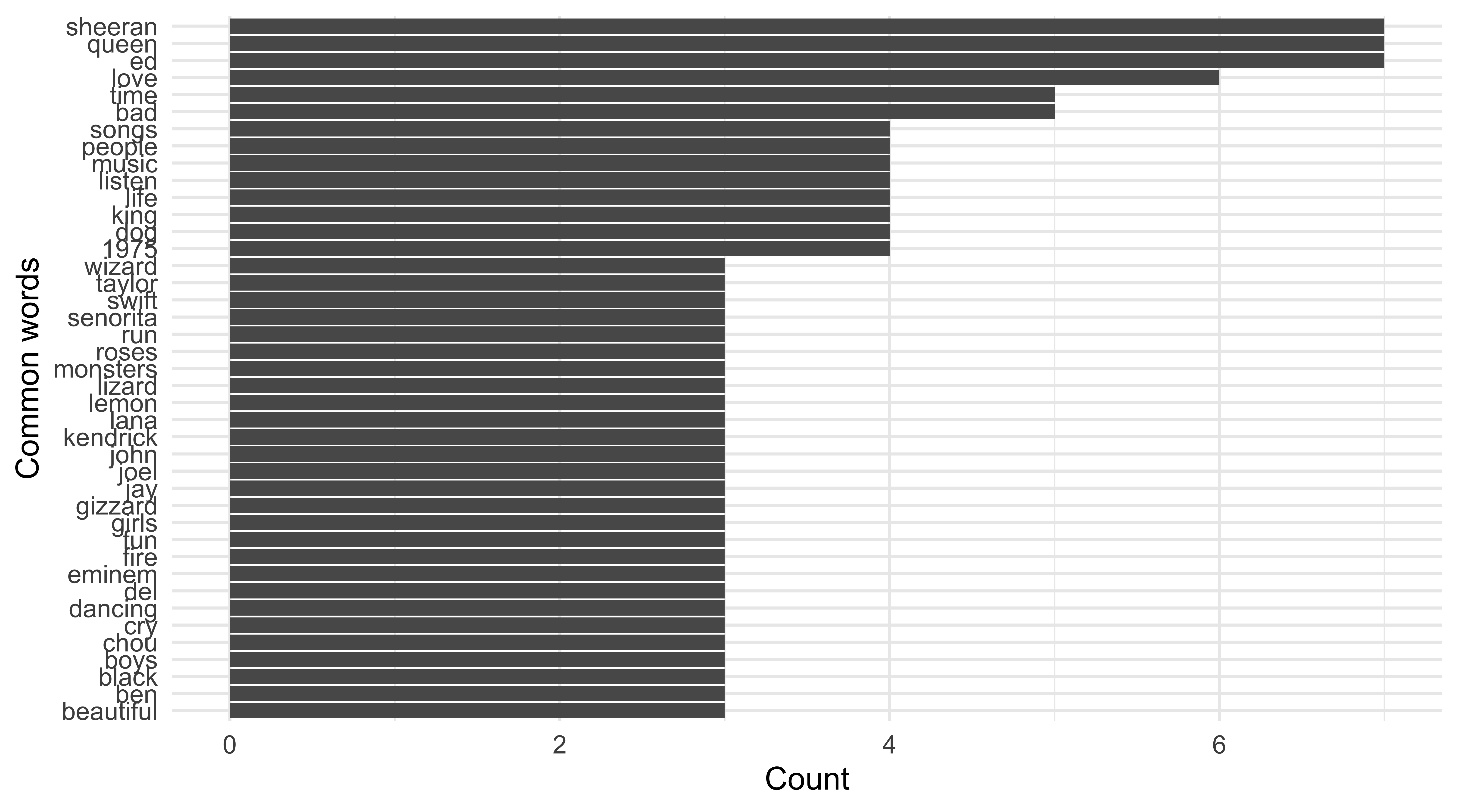
Top 20 common words in songstop20_songs <- listening %>%
  unnest_tokens(word, songs) %>%
  anti_join(stop_words) %>%
  filter(
    !(word %in% c("1", "2", "3", "4", "5"))
    ) %>%
  count(word) %>%
  top_n(20)

top20_songs %>%
  arrange(desc(n))

## # A tibble: 41 x 2
##    word        n
##    <chr>   <int>
##  1 ed          7
##  2 queen       7
##  3 sheeran     7
##  4 love        6
##  5 bad         5
##  6 time        5
##  7 1975        4
##  8 dog         4
##  9 king        4
## 10 life        4
## # … with 31 more rows
20 / 59

Visualizing commonalities: bar chart

21 / 59

... the code

ggplot(top20_songs, aes(x = fct_reorder(word, n), y = n)) +
  geom_col() +
  labs(x = "Common words", y = "Count") +
  coord_flip()

22 / 59

Visualizing commonalities: wordcloud

23 / 59

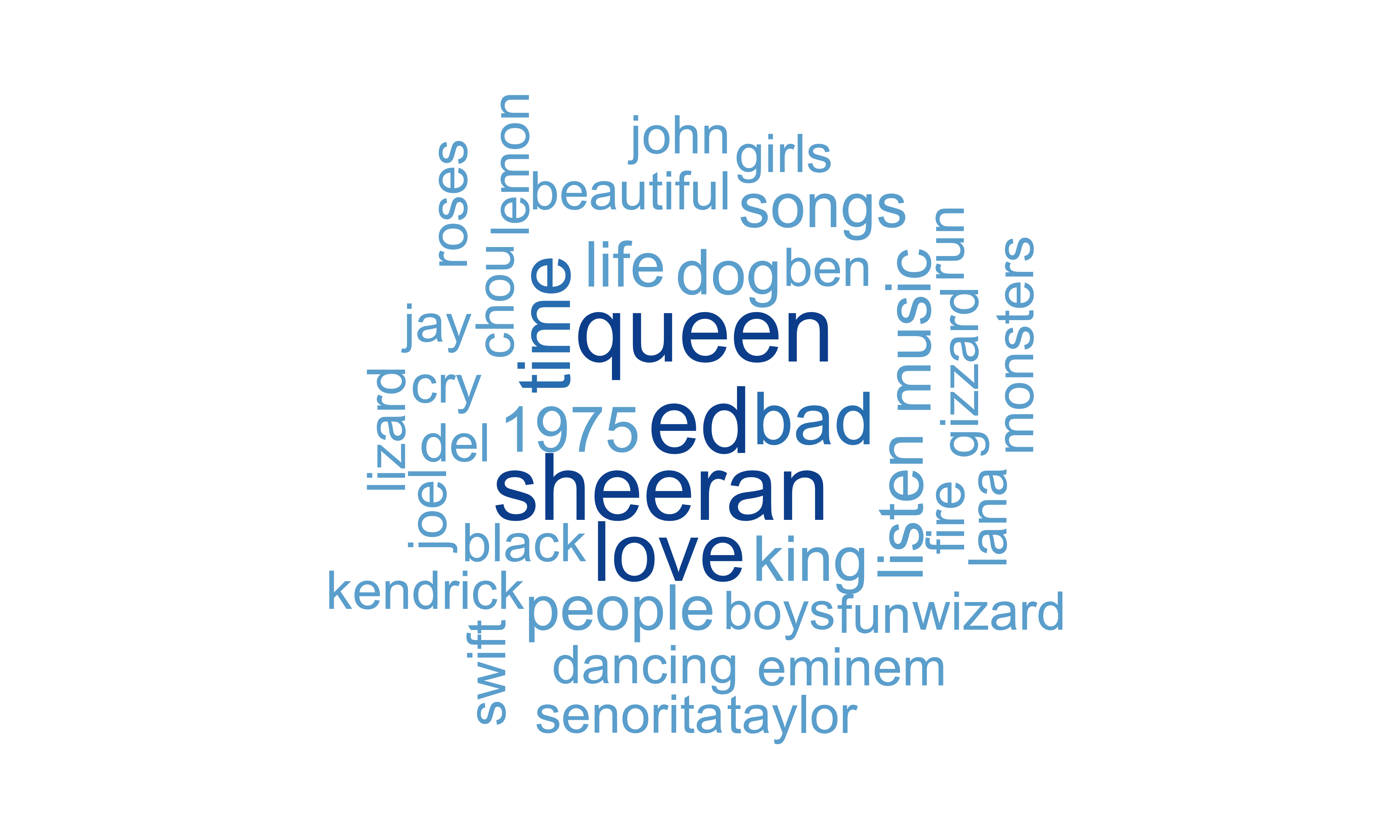
... and the code

set.seed(1234)
wordcloud(words = top20_songs$word, 
          freq = top20_songs$n, 
          colors = brewer.pal(5,"Blues"),
          random.order = FALSE)

24 / 59

Ok, so people like Ed Sheeran!

str_subset(listening$songs, "Sheeran")

## [1] "Mess by Ed Sheeran, Take me back to london by Ed Sheeran and Sounds of the Skeng by Stormzy"                
## [2] "Ed Sheeran- I don't care, beautiful people, don't"                                                          
## [3] "Truth Hurts by Lizzo , Wetsuit by The Vaccines , Beautiful People by Ed Sheeran"                            
## [4] "Sounds of the Skeng - Stormzy, Venom - Eminem, Take me back to london - Ed Sheeran, I see fire - Ed Sheeran"

25 / 59

But I had to ask...

26 / 59

But I had to ask...

What is 1975?

26 / 59

But I had to ask...

What is 1975?

str_subset(listening$songs, "1975")

## [1] "Hate Me (Sometimes) - Stand Atlantic; Edge of Seventeen - Stevie Nicks; It's Not Living (If It's Not With You) - The 1975; People - The 1975; Hypersonic Missiles - Sam Fender"
## [2] "Chocolate by the 1975, sanctuary by Joji, A young understating by Sundara Karma"                                                                                               
## [3] "Lauv - I'm lonely, kwassa - good life, the 1975 - sincerity is scary"

26 / 59

Analyzing lyrics of one artist

27 / 59

Let's get more data

We'll use the genius package to get song lyric data from Genius.

genius_album(): download lyrics for an entire album
add_genius(): download lyrics for multiple albums

28 / 59

Ed's most recent-ish albums

artist_albums <- tribble(
  ~artist,      ~album,
  "Ed Sheeran", "No.6 Collaborations Project",
  "Ed Sheeran", "Divide",
  "Ed Sheeran", "Multiply",
  "Ed Sheeran", "Plus",
)
sheeran <- artist_albums %>%
  add_genius(artist, album)

29 / 59

Songs in the four albums

	album	track_title
1	No.6 Collaborations Project	Beautiful People (Ft. Khalid)
2	No.6 Collaborations Project	South of the Border (Ft. Camila Cabello & Cardi B)
3	No.6 Collaborations Project	Cross Me (Ft. Chance the Rapper & PnB Rock)
4	No.6 Collaborations Project	Take Me Back to London (Ft. Stormzy)
5	No.6 Collaborations Project	Best Part of Me (Ft. YEBBA)
6	No.6 Collaborations Project	I Don't Care by Ed Sheeran & Justin Bieber
7	No.6 Collaborations Project	Antisocial by Ed Sheeran & Travis Scott
8	No.6 Collaborations Project	Remember the Name (Ft. 50 Cent & Eminem)
9	No.6 Collaborations Project	Feels (Ft. J Hus & Young Thug)
10	No.6 Collaborations Project	Put It All on Me (Ft. Ella Mai)

30 / 59

How long are Ed Sheeran's songs?

Length measured by number of lines

sheeran %>%
  count(track_title, sort = TRUE)

## # A tibble: 73 x 2
##    track_title                                            n
##    <chr>                                              <int>
##  1 Take It Back                                         101
##  2 The Man                                               96
##  3 Cross Me (Ft.&nbsp;Chance&nbsp;the Rapper & PnB&nbsp;Rock)           95
##  4 You Need Me, I Don't Need You                         94
##  5 Shape of You                                          91
##  6 Nina                                                  89
##  7 Remember the Name (Ft.&nbsp;50&nbsp;Cent & Eminem)              77
##  8 South of the Border (Ft.&nbsp;Camila&nbsp;Cabello & Cardi&nbsp;B)    77
##  9 Bloodstream                                           76
## 10 Take Me Back to London (Ft.&nbsp;Stormzy)                  75
## # … with 63 more rows

31 / 59

Tidy up your lyrics!

sheeran_lyrics <- sheeran %>%
  unnest_tokens(word, lyric)
sheeran_lyrics

## # A tibble: 30,023 x 6
##    artist    album               track_title           track_n  line word  
##    <chr>     <chr>               <chr>                   <int> <int> <chr> 
##  1 Ed Sheer… No.6 Collaboration… Beautiful People (Ft…       1     1 we    
##  2 Ed Sheer… No.6 Collaboration… Beautiful People (Ft…       1     1 are   
##  3 Ed Sheer… No.6 Collaboration… Beautiful People (Ft…       1     1 we    
##  4 Ed Sheer… No.6 Collaboration… Beautiful People (Ft…       1     1 are   
##  5 Ed Sheer… No.6 Collaboration… Beautiful People (Ft…       1     1 we    
##  6 Ed Sheer… No.6 Collaboration… Beautiful People (Ft…       1     1 are   
##  7 Ed Sheer… No.6 Collaboration… Beautiful People (Ft…       1     2 l.a   
##  8 Ed Sheer… No.6 Collaboration… Beautiful People (Ft…       1     2 on    
##  9 Ed Sheer… No.6 Collaboration… Beautiful People (Ft…       1     2 a     
## 10 Ed Sheer… No.6 Collaboration… Beautiful People (Ft…       1     2 satur…
## # … with 30,013 more rows

32 / 59

What are the most common words?

sheeran_lyrics %>%
  count(word, sort = TRUE)

## # A tibble: 2,830 x 2
##    word      n
##    <chr> <int>
##  1 i      1161
##  2 you    1013
##  3 the     992
##  4 and     886
##  5 my      823
##  6 me      689
##  7 to      556
##  8 in      517
##  9 a       500
## 10 on      408
## # … with 2,820 more rows

33 / 59

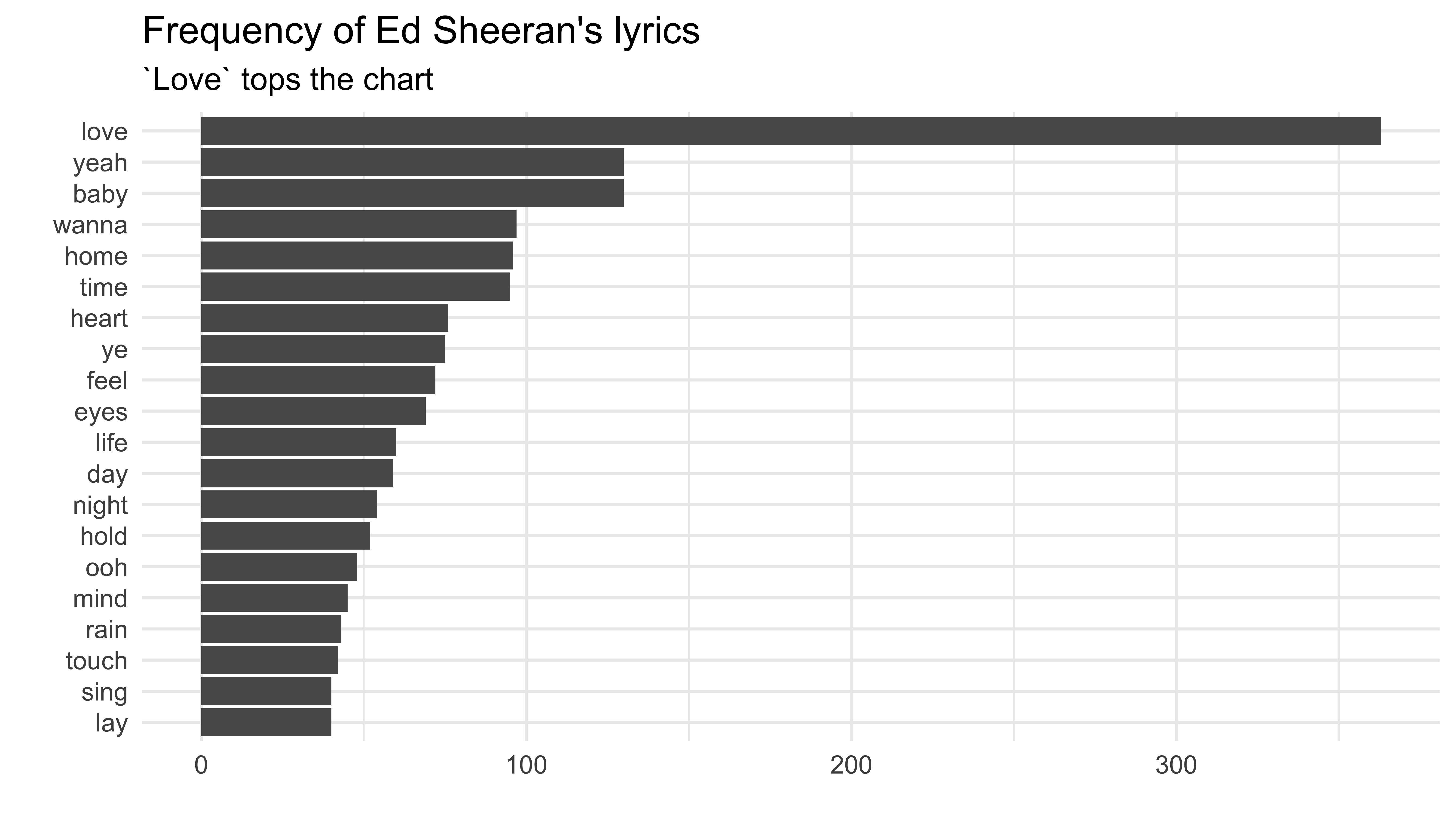
What a romantic!

sheeran_lyrics %>%
  anti_join(stop_words) %>%
  count(word, sort = TRUE)

## Joining, by = "word"

## # A tibble: 2,413 x 2
##    word      n
##    <chr> <int>
##  1 love    363
##  2 baby    130
##  3 yeah    130
##  4 wanna    97
##  5 home     96
##  6 time     95
##  7 heart    76
##  8 ye       75
##  9 feel     72
## 10 eyes     69
## # … with 2,403 more rows

34 / 59

35 / 59

... and the code

sheeran_lyrics %>%
  anti_join(stop_words) %>%
  count(word)%>%
  top_n(20) %>%
  ggplot(aes(fct_reorder(word, n), n)) +
    geom_col() +
    labs(title = "Frequency of Ed Sheeran's lyrics",
         subtitle = "`Love` tops the chart",
         y = "",
         x = "") +
    coord_flip()

36 / 59

Sentiment analysis

37 / 59

Sentiment analysis

One way to analyze the sentiment of a text is to consider the text as a combination of its individual words
and the sentiment content of the whole text as the sum of the sentiment content of the individual words

38 / 59

Sentiment lexicons

get_sentiments("afinn")

## # A tibble: 2,477 x 2
##    word       value
##    <chr>      <dbl>
##  1 abandon       -2
##  2 abandoned     -2
##  3 abandons      -2
##  4 abducted      -2
##  5 abduction     -2
##  6 abductions    -2
##  7 abhor         -3
##  8 abhorred      -3
##  9 abhorrent     -3
## 10 abhors        -3
## # … with 2,467 more rows

get_sentiments("bing")

## # A tibble: 6,786 x 2
##    word        sentiment
##    <chr>       <chr>    
##  1 2-faces     negative 
##  2 abnormal    negative 
##  3 abolish     negative 
##  4 abominable  negative 
##  5 abominably  negative 
##  6 abominate   negative 
##  7 abomination negative 
##  8 abort       negative 
##  9 aborted     negative 
## 10 aborts      negative 
## # … with 6,776 more rows

39 / 59

Sentiment lexicons

get_sentiments("nrc")

## # A tibble: 13,901 x 2
##    word        sentiment
##    <chr>       <chr>    
##  1 abacus      trust    
##  2 abandon     fear     
##  3 abandon     negative 
##  4 abandon     sadness  
##  5 abandoned   anger    
##  6 abandoned   fear     
##  7 abandoned   negative 
##  8 abandoned   sadness  
##  9 abandonment anger    
## 10 abandonment fear     
## # … with 13,891 more rows

get_sentiments("loughran")

## # A tibble: 4,150 x 2
##    word         sentiment
##    <chr>        <chr>    
##  1 abandon      negative 
##  2 abandoned    negative 
##  3 abandoning   negative 
##  4 abandonment  negative 
##  5 abandonments negative 
##  6 abandons     negative 
##  7 abdicated    negative 
##  8 abdicates    negative 
##  9 abdicating   negative 
## 10 abdication   negative 
## # … with 4,140 more rows

40 / 59

Categorizing sentiments

41 / 59

Sentiments in Sheeran's lyrics

sheeran_lyrics %>%
  inner_join(get_sentiments("bing")) %>%
  count(sentiment, word, sort = TRUE)

## Joining, by = "word"

## # A tibble: 359 x 3
##    sentiment word          n
##    <chr>     <chr>     <int>
##  1 positive  love        363
##  2 positive  like        202
##  3 positive  right        46
##  4 positive  well         33
##  5 positive  darling      31
##  6 positive  lover        30
##  7 positive  loved        29
##  8 negative  fall         25
##  9 positive  beautiful    23
## 10 negative  cold         22
## # … with 349 more rows

42 / 59

Goal: Find the top 10 most common words with positive and negative sentiments.

43 / 59

Step 1: Top 10 words for each sentiment

sheeran_lyrics %>%
  inner_join(get_sentiments("bing")) %>%
  count(sentiment, word) %>%
  group_by(sentiment) %>%
  top_n(10)

## # A tibble: 20 x 3
## # Groups:   sentiment [2]
##    sentiment word          n
##    <chr>     <chr>     <int>
##  1 negative  bad          16
##  2 negative  break        21
##  3 negative  cold         22
##  4 negative  drunk        19
##  5 negative  fall         25
##  6 negative  falling      22
##  7 negative  hurting      16
##  8 negative  miss         20
##  9 negative  pain         19
## 10 negative  shit         20
## 11 positive  beautiful    23
## 12 positive  better       19
## 13 positive  darling      31
## 14 positive  free         22
## 15 positive  like        202
## 16 positive  love        363
## 17 positive  loved        29
## 18 positive  lover        30
## 19 positive  right        46
## 20 positive  well         33

44 / 59

Step 2: `ungroup()`

sheeran_lyrics %>%
  inner_join(get_sentiments("bing")) %>%
  count(sentiment, word) %>%
  group_by(sentiment) %>%
  top_n(10) %>%
  ungroup()

## # A tibble: 20 x 3
##    sentiment word          n
##    <chr>     <chr>     <int>
##  1 negative  bad          16
##  2 negative  break        21
##  3 negative  cold         22
##  4 negative  drunk        19
##  5 negative  fall         25
##  6 negative  falling      22
##  7 negative  hurting      16
##  8 negative  miss         20
##  9 negative  pain         19
## 10 negative  shit         20
## 11 positive  beautiful    23
## 12 positive  better       19
## 13 positive  darling      31
## 14 positive  free         22
## 15 positive  like        202
## 16 positive  love        363
## 17 positive  loved        29
## 18 positive  lover        30
## 19 positive  right        46
## 20 positive  well         33

45 / 59

Step 3: Save the result

sheeran_top10 <- sheeran_lyrics %>%
  inner_join(get_sentiments("bing")) %>%
  count(sentiment, word) %>%
  group_by(sentiment) %>%
  top_n(10) %>%
  ungroup()

46 / 59

Goal: Visualize the top 10 most common words with positive and negative sentiments.

47 / 59

Step 1: Create a bar chart

sheeran_top10 %>%
  ggplot(aes(x = word, y = n, fill = sentiment)) +
  geom_col()

48 / 59

Step 2: Order bars by frequency

sheeran_top10 %>%
  ggplot(aes(x = fct_reorder(word, n), y = n, fill = sentiment)) +
  geom_col()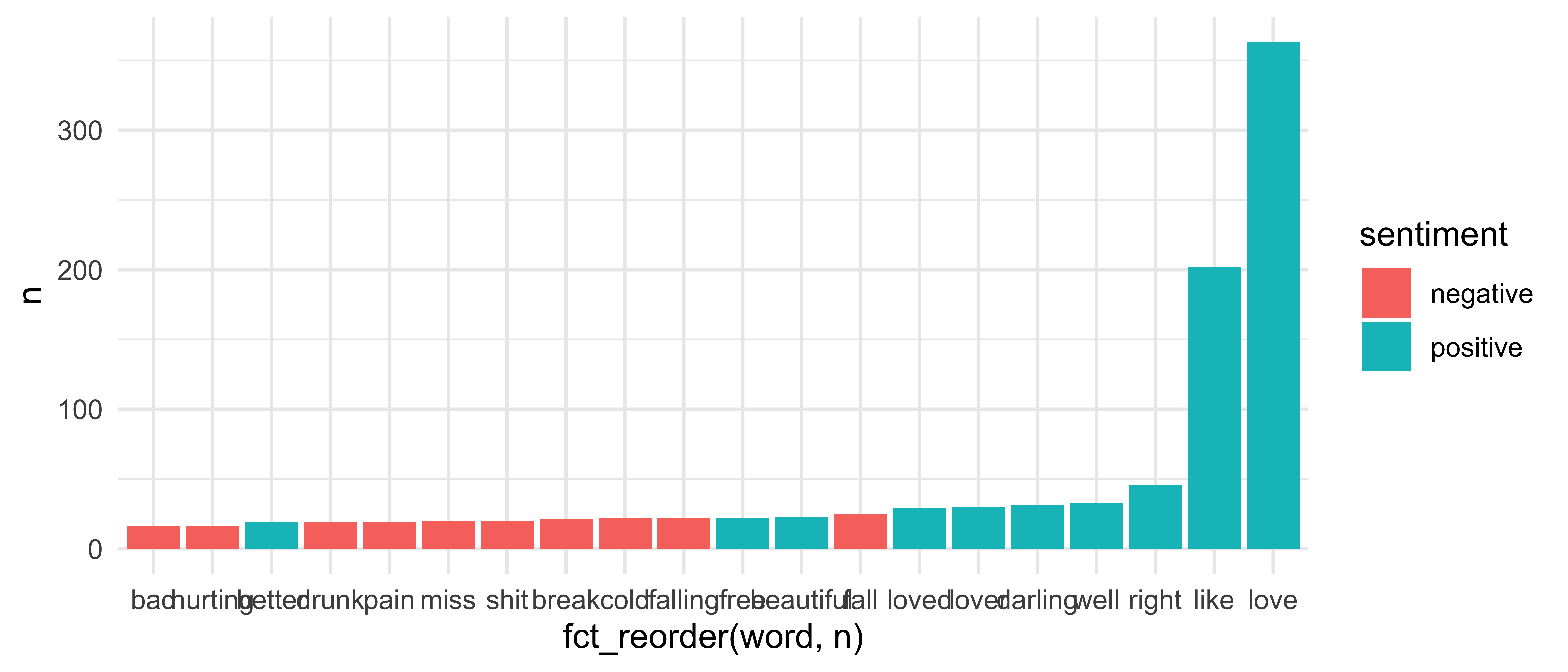

49 / 59

sheeran_top10 %>%
  ggplot(aes(x = fct_reorder(word, n), y = n, fill = sentiment)) +
  geom_col() +
  facet_wrap(~ sentiment)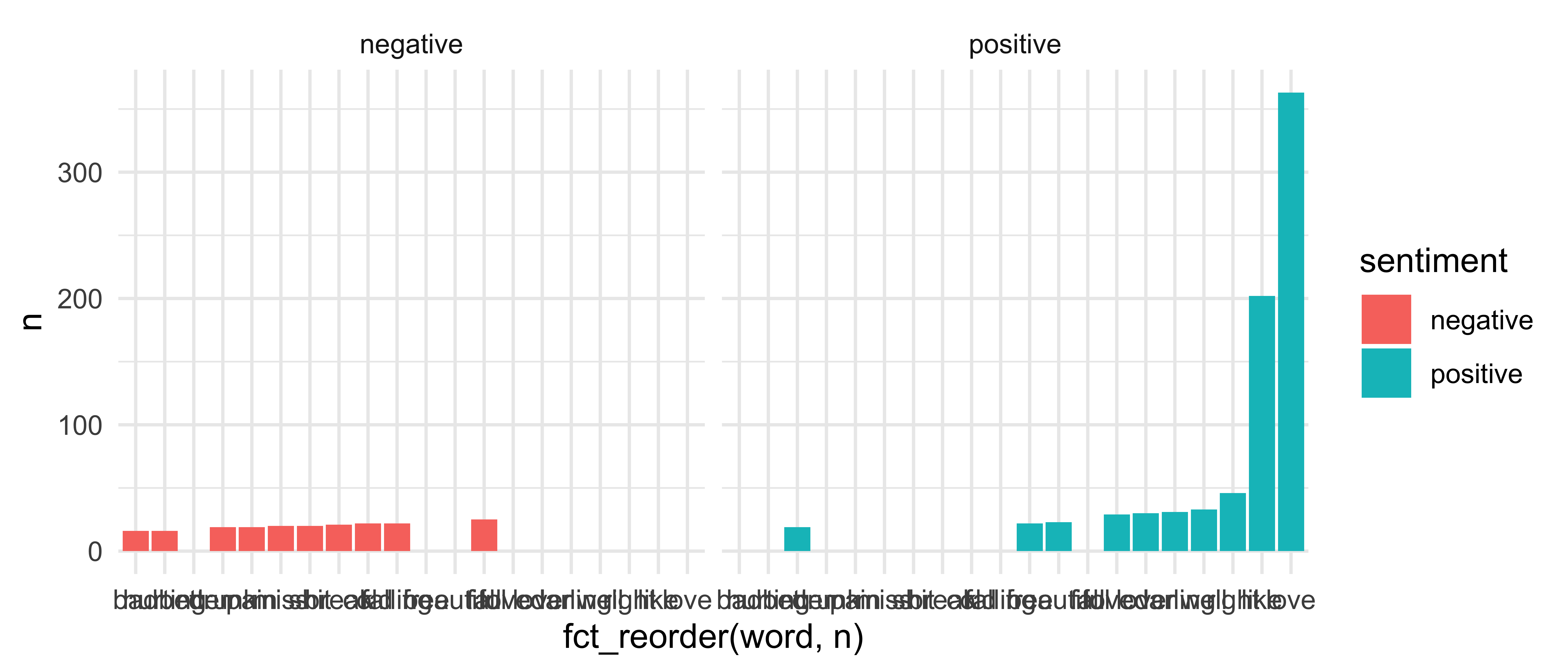

50 / 59

Step 4: Free the scales!

sheeran_top10 %>%
  ggplot(aes(x = fct_reorder(word, n), y = n, fill = sentiment)) +
  geom_col() +
  facet_wrap(~ sentiment, scales = "free")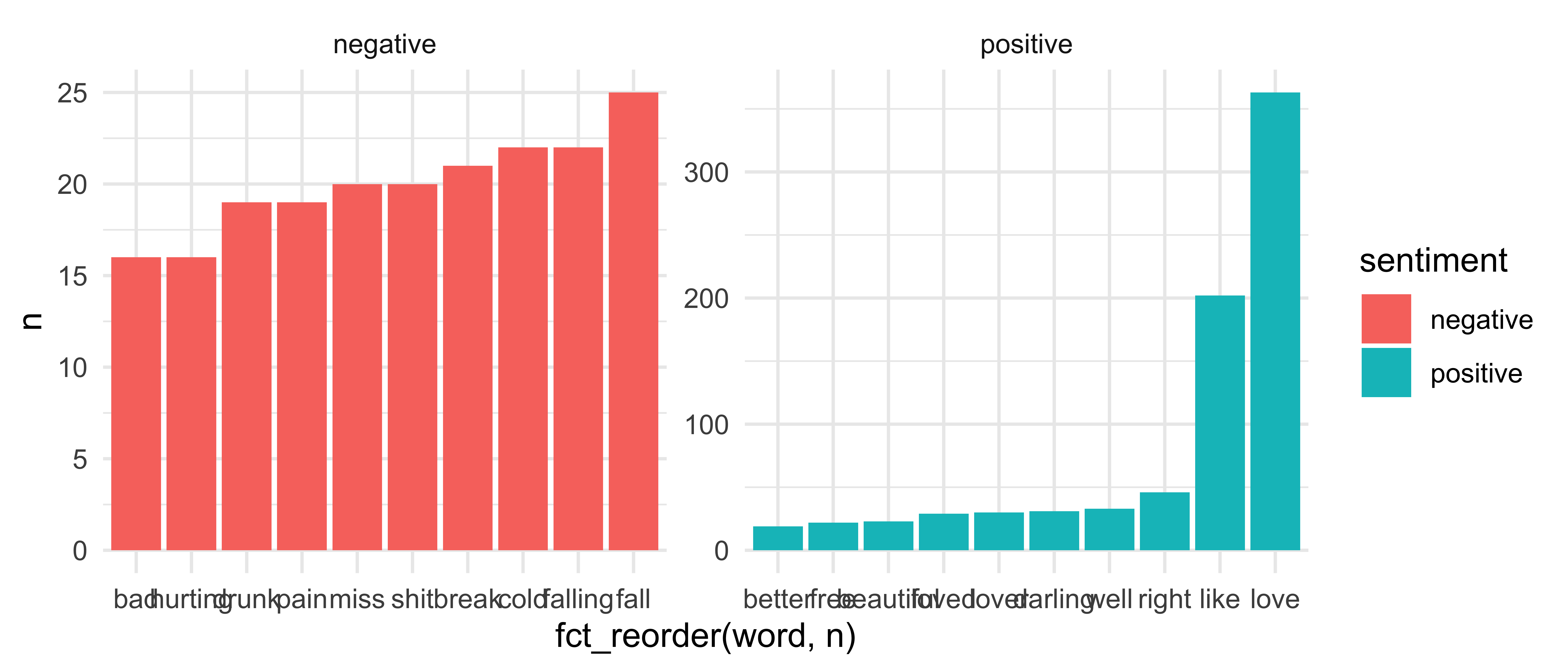

51 / 59

Step 4: Flip the coordinates

sheeran_top10 %>%
  ggplot(aes(x = fct_reorder(word, n), y = n, fill = sentiment)) +
  geom_col() +
  facet_wrap(~ sentiment, scales = "free") +
  coord_flip()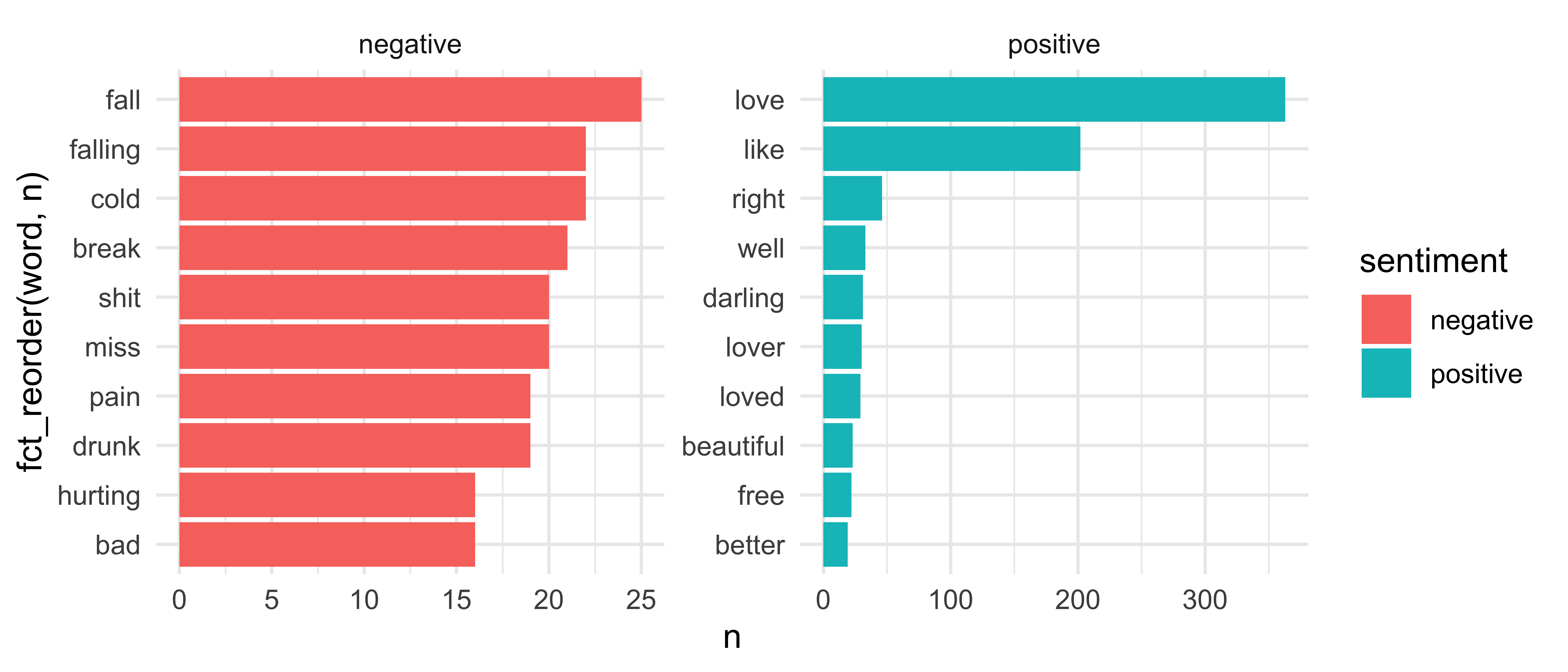

52 / 59

Step 5: Clean up labels

sheeran_top10 %>%
  ggplot(aes(x = fct_reorder(word, n), y = n, fill = sentiment)) +
  geom_col() +
  facet_wrap(~ sentiment, scales = "free") +
  coord_flip() +
  labs(title = "Sentiments in Ed Sheeran's lyrics", x = "", y = "")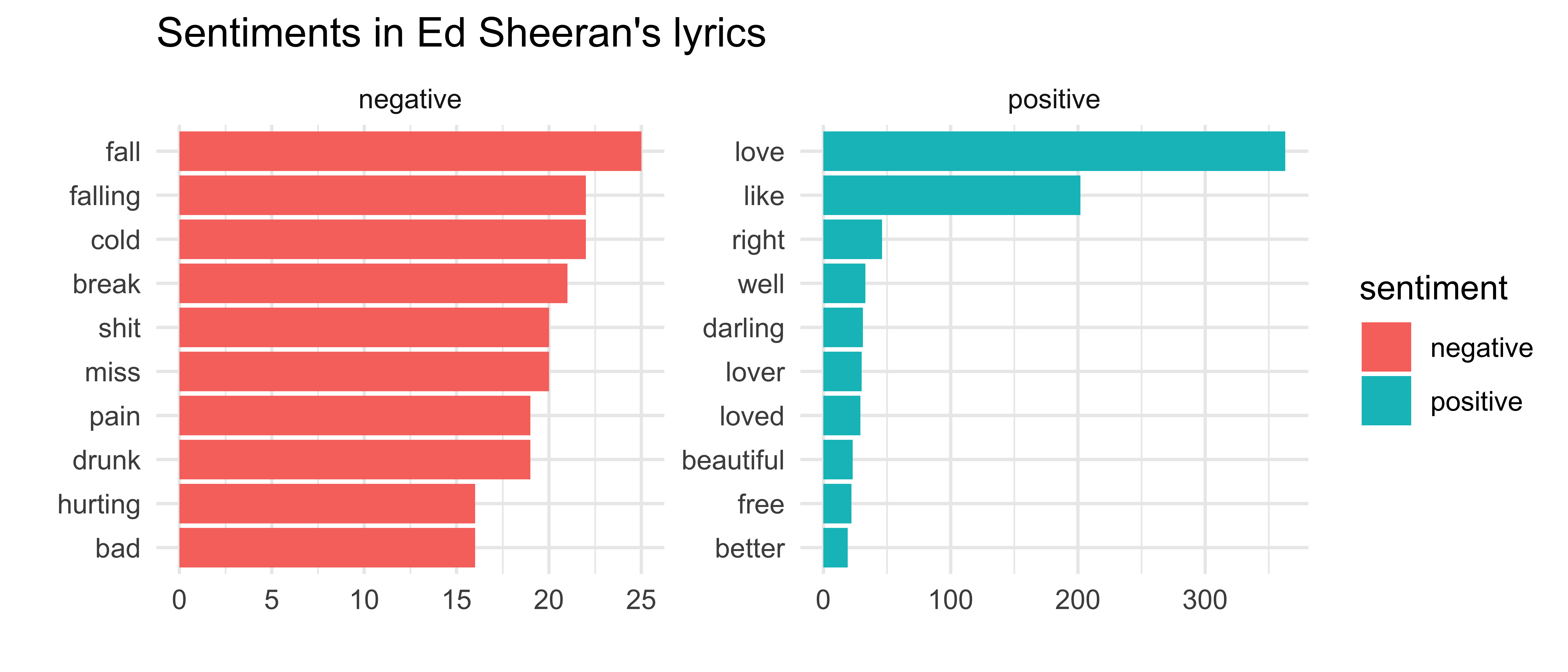

53 / 59

Step 6: Remove redundant info

sheeran_top10 %>%
  ggplot(aes(x = fct_reorder(word, n), y = n, fill = sentiment)) +
  geom_col() +
  facet_wrap(~ sentiment, scales = "free") +
  coord_flip() +
  labs(title = "Sentiments in Ed Sheeran's lyrics", x = "", y = "") +
  guides(fill = FALSE)

54 / 59

Scoring sentiments

55 / 59

Assign a sentiment score

sheeran_lyrics %>%
  anti_join(stop_words) %>%
  left_join(get_sentiments("afinn"))

## Joining, by = "word"Joining, by = "word"

## # A tibble: 9,186 x 7
##    artist   album           track_title        track_n  line word     value
##    <chr>    <chr>           <chr>                <int> <int> <chr>    <dbl>
##  1 Ed Shee… No.6 Collabora… Beautiful People …       1     2 l.a         NA
##  2 Ed Shee… No.6 Collabora… Beautiful People …       1     2 saturday    NA
##  3 Ed Shee… No.6 Collabora… Beautiful People …       1     2 night       NA
##  4 Ed Shee… No.6 Collabora… Beautiful People …       1     2 summer      NA
##  5 Ed Shee… No.6 Collabora… Beautiful People …       1     3 sundown     NA
##  6 Ed Shee… No.6 Collabora… Beautiful People …       1     4 lamborg…    NA
##  7 Ed Shee… No.6 Collabora… Beautiful People …       1     4 rented      NA
##  8 Ed Shee… No.6 Collabora… Beautiful People …       1     4 hummers     NA
##  9 Ed Shee… No.6 Collabora… Beautiful People …       1     5 party's     NA
## 10 Ed Shee… No.6 Collabora… Beautiful People …       1     5 headin      NA
## # … with 9,176 more rows

56 / 59

sheeran_lyrics %>%
  anti_join(stop_words) %>%
  left_join(get_sentiments("afinn")) %>%
  filter(!is.na(value)) %>%
  group_by(album) %>%
  summarise(total_sentiment = sum(value)) %>%
  arrange(total_sentiment)

## # A tibble: 4 x 2
##   album                       total_sentiment
##   <chr>                                 <dbl>
## 1 No.6 Collaborations Project             102
## 2 Multiply                                112
## 3 Plus                                    218
## 4 Divide                                  378

57 / 59

58 / 59

Acknowledgements

Julia Silge: https://github.com/juliasilge/tidytext-tutorial
Julia Silge and David Robinson: https://www.tidytextmining.com/
Josiah Parry: https://github.com/JosiahParry/genius

59 / 59

Announcements

This week's recap email will have instructions on checking/confirming your marks so far on Learn

Don't forget to turn in peer feedback for projects (for your team and other teams) by 17:00 today

HW 10 due Friday: You can use lower number of bootstrap samples, e.g. 1000.

OQ 10 due Friday: Last item due!

Making your project repo public (optional)

2 / 59

Help

Keyboard shortcuts

↑, ←, Pg Up, k

Go to previous slide

↓, →, Pg Dn, Space, j

Go to next slide

Home

Go to first slide

End

Go to last slide

Number + Return

Go to specific slide

b / m / f

Toggle blackout / mirrored / fullscreen mode

Clone slideshow

Toggle presenter mode

Restart the presentation timer

?, h

Toggle this help

Text analysis 📃

Dr. Çetinkaya-Rundel

Announcements

Piazza awards!

Stickers!

Save the date!

ASA DataFest @ EDI

Tidytext analysis

Packages

Tidytext

What is tidy text?

What is tidy text?

What is tidy text?

What are you listening to?

From the "Getting to know you" survey

Looking for commonalities

Stop words

English stop words

Spanish stop words

Various lexicons

Back to: Looking for commonalities

Top 20 common words in songs

Visualizing commonalities: bar chart

Visualizing commonalities: wordcloud

Ok, so people like Ed Sheeran!

But I had to ask...

But I had to ask...

But I had to ask...

Analyzing lyrics of one artist

Let's get more data

Ed's most recent-ish albums

Songs in the four albums

How long are Ed Sheeran's songs?

Tidy up your lyrics!

What are the most common words?

What a romantic!

Sentiment analysis

Sentiment analysis

Sentiment lexicons

Sentiment lexicons

Categorizing sentiments

Sentiments in Sheeran's lyrics

Step 1: Top 10 words for each sentiment

Step 2: ungroup()

Step 3: Save the result

Step 1: Create a bar chart

Step 2: Order bars by frequency

Step 3: Facet by sentiment

Step 4: Free the scales!

Step 4: Flip the coordinates

Step 5: Clean up labels

Step 6: Remove redundant info

Scoring sentiments

Assign a sentiment score

Acknowledgements

Announcements

Help

Text analysis
📃

Step 2: `ungroup()`