Fundamentals of data and data visualization 
 📊Dr. Çetinkaya-Rundel1 / 55

Week 2

Preparing for tomorrow's workshop: Make sure you have completed Lab 01, and ask questions if you get stuck, complete survey asap
Workshop tomorrow: Individual to give you some more practice on your own + hold off on setting teams till after drop/add
Due this week: HW 01 (Wednesday) + OQ 01 (Friday)
- Neither of these are graded, but you're strongly recommended to complete them
Student hours for this week only: After class today + no student hours on Tuesday (but I'll be answering questions on Piazza)
Thanks to all asking and answering questions on Piazza!

Any questions?

2 / 55

Getting help in R

3 / 55

Reading help files

Source: http://socviz.co/appendix.html#a-little-more-about-r

4 / 55

Asking good questions

Good: Describe your intention and include your code and the error
Better: Describe your intention and create a minimum working example
Best: Write a reproducible example (reprex) -- we'll introduce this concept more formally and teach you the tools for it a little later in the semester

5 / 55

Asking good questions

Good: Describe your intention and include your code and the error
Better: Describe your intention and create a minimum working example
Best: Write a reproducible example (reprex) -- we'll introduce this concept more formally and teach you the tools for it a little later in the semester

Use code formatting
For issues with R code: copy / paste your code and resulting error, don't use screenshots

5 / 55

Exploratory data analysis

6 / 55

What is EDA?

Exploratory data analysis (EDA) is an aproach to analyzing data sets to summarize its main characteristics.
Often, this is visual. That's what we're focusing on today.
But we might also calculate summary statistics and perform data wrangling/manipulation/transformation at (or before) this stage of the analysis. That's what we'll focus on next.

7 / 55

Data visualization

8 / 55

Data visualization

"The simple graph has brought more information to the data analyst’s mind than any other device." — John Tukey

Data visualization is the creation and study of the visual representation of data.
There are many tools for visualizing data (R is one of them), and many approaches/systems within R for making data visualizations (ggplot2 is one of them, and that's what we're going to use).

9 / 55

ggplot2 $\in$ tidyverse

ggplot2 is tidyverse's data visualization package
The gg in "ggplot2" stands for Grammar of Graphics
It is inspired by the book Grammar of Graphics by Leland Wilkinson

10 / 55

Grammar of Graphics

A grammar of graphics is a tool that enables us to concisely describe the components of a graphic

Source: BloggoType

11 / 55

ggplot(data = starwars, mapping = aes(x = height, y = mass)) +
  geom_point() +
  labs(title = "Mass vs. height of Starwars characters",
       x = "Height (cm)", y = "Weight (kg)")

## Warning: Removed 28 rows containing missing values (geom_point).

12 / 55

What are the functions doing the plotting?
What is the dataset being plotted?
Which variable is on the x-axis and which variable is on the y-axis?
What does the warning mean?

ggplot(data = starwars, mapping = aes(x = height, y = mass)) +
  geom_point() +
  labs(
    title = "Mass vs. height of Starwars characters",
    x = "Height (cm)", 
    y = "Weight (kg)"
    )

## Warning: Removed 28 rows containing missing values (geom_point).

13 / 55

What does geom_smooth() do?

ggplot(data = starwars, mapping = aes(x = height, y = mass)) +
  geom_point() +
  geom_smooth() +
  labs(title = "Mass vs. height of Starwars characters",
       x = "Height (cm)", y = "Weight (kg)")

14 / 55

Hello ggplot2!

ggplot() is the main function in ggplot2
Plots are constructed in layers
Structure of the code for plots can be summarized as

ggplot(data = [dataset], 
       mapping = aes(x = [x-variable], y = [y-variable])) +
   geom_xxx() +
   other options

To use ggplot2 functions, first load tidyverse

library(tidyverse)

For help with the ggplot2, see ggplot2.tidyverse.org

15 / 55

Visualizing Star Wars

16 / 55

Dataset terminology

Each row is an observation
Each column is a variable

starwars

## # A tibble: 87 x 13
##    name  height  mass hair_color skin_color eye_color birth_year gender
##    <chr>  <int> <dbl> <chr>      <chr>      <chr>          <dbl> <chr> 
##  1 Luke…    172    77 blond      fair       blue            19   male  
##  2 C-3PO    167    75 <NA>       gold       yellow         112   <NA>  
##  3 R2-D2     96    32 <NA>       white, bl… red             33   <NA>  
##  4 Dart…    202   136 none       white      yellow          41.9 male  
##  5 Leia…    150    49 brown      light      brown           19   female
##  6 Owen…    178   120 brown, gr… light      blue            52   male  
##  7 Beru…    165    75 brown      light      blue            47   female
##  8 R5-D4     97    32 <NA>       white, red red             NA   <NA>  
##  9 Bigg…    183    84 black      light      brown           24   male  
## 10 Obi-…    182    77 auburn, w… fair       blue-gray       57   male  
## # … with 77 more rows, and 5 more variables: homeworld <chr>,
## #   species <chr>, films <list>, vehicles <list>, starships <list>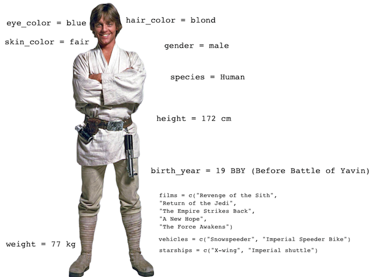

17 / 55

Luke Skywalker

luke-skywalker

18 / 55

What's in the Star Wars data?

Take a glimpse at the data:

glimpse(starwars)

## Observations: 87
## Variables: 13
## $ name       <chr> "Luke Skywalker", "C-3PO", "R2-D2", "Darth Vader", "L…
## $ height     <int> 172, 167, 96, 202, 150, 178, 165, 97, 183, 182, 188, …
## $ mass       <dbl> 77.0, 75.0, 32.0, 136.0, 49.0, 120.0, 75.0, 32.0, 84.…
## $ hair_color <chr> "blond", NA, NA, "none", "brown", "brown, grey", "bro…
## $ skin_color <chr> "fair", "gold", "white, blue", "white", "light", "lig…
## $ eye_color  <chr> "blue", "yellow", "red", "yellow", "brown", "blue", "…
## $ birth_year <dbl> 19.0, 112.0, 33.0, 41.9, 19.0, 52.0, 47.0, NA, 24.0, …
## $ gender     <chr> "male", NA, NA, "male", "female", "male", "female", N…
## $ homeworld  <chr> "Tatooine", "Tatooine", "Naboo", "Tatooine", "Alderaa…
## $ species    <chr> "Human", "Droid", "Droid", "Human", "Human", "Human",…
## $ films      <list> [<"Revenge of the Sith", "Return of the Jedi", "The …
## $ vehicles   <list> [<"Snowspeeder", "Imperial Speeder Bike">, <>, <>, <…
## $ starships  <list> [<"X-wing", "Imperial shuttle">, <>, <>, "TIE Advanc…

19 / 55

What's in the Star Wars data?

How many rows and columns does this dataset have? What does each row represent? What does each column represent?

?starwars

20 / 55

Mass vs. height

ggplot(data = starwars, mapping = aes(x = height, y = mass)) +
  geom_point()

## Warning: Removed 28 rows containing missing values (geom_point).

21 / 55

What's that warning?

Not all characters have height and mass information (hence 28 of them not plotted)

## Warning: Removed 28 rows containing missing values (geom_point).

Going forward I'll supress the warning to save room on slides, but it's important to note it

22 / 55

Labels

ggplot(data = starwars, mapping = aes(x = height, y = mass)) +
  geom_point() +
  labs(title = "Mass vs. height of Starwars characters",
       x = "Height (cm)", y = "Weight (kg)")

23 / 55

Mass vs. height

How would you describe this relationship? What other variables would help us understand data points that don't follow the overall trend? Who is the not so tall but really chubby character?

24 / 55

Jabba!

25 / 55

Additional variables

We can map additional variables to various features of the plot:

aesthetics
- shape
- colour
- size
- alpha (transparency)
faceting: small multiples displaying different subsets

26 / 55

Aesthetics

27 / 55

Aesthetics options

Visual characteristics of plotting characters that can be mapped to a specific variable in the data are

color
size
shape
alpha (transparency)

28 / 55

Mass vs. height + gender

ggplot(data = starwars, 
       mapping = aes(x = height, y = mass, color = gender)) +
  geom_point()

29 / 55

Mass vs. height + gender

ggplot(data = starwars, 
       mapping = aes(x = height, y = mass, color = gender, 
                     size = birth_year)) +
  geom_point()

30 / 55

Mass vs. height + gender

Let's now increase the size of all points not based on the values of a variable in the data:

ggplot(data = starwars, mapping = aes(x = height, y = mass, color = gender)) +
  geom_point(size = 2)

31 / 55

Aesthetics summary

Continuous variable are measured on a continuous scale
Discrete variables are measured (or often counted) on a discrete scale

aesthetics	discrete	continuous
color	rainbow of colors	gradient
size	discrete steps	linear mapping between radius and value
shape	different shape for each	shouldn't (and doesn't) work

Use aesthetics for mapping features of a plot to a variable, define the features in the geom for customization not mapped to a variable

32 / 55

Faceting

33 / 55

Faceting

Smaller plots that display different subsets of the data
Useful for exploring conditional relationships and large data

34 / 55

ggplot(data = starwars, mapping = aes(x = height, y = mass)) +
  facet_grid(. ~ gender) +
  geom_point() +
  labs(title = "Mass vs. height of Starwars characters",
       subtitle = "Faceted by gender")

35 / 55

Dive further...

In the next few slides describe what each plot displays. Think about how the code relates to the output.

36 / 55

Dive further...

In the next few slides describe what each plot displays. Think about how the code relates to the output.

The plots in the next few slides do not have proper titles, axis labels, etc. because we want you to figure out what's happening in the plots. But you should always label your plots!

36 / 55

ggplot(data = starwars, mapping = aes(x = height, y = mass)) +
  geom_point() +
  facet_grid(gender ~ .)

37 / 55

ggplot(data = starwars, mapping = aes(x = height, y = mass)) +
  geom_point() +
  facet_grid(. ~ gender)

38 / 55

ggplot(data = starwars, mapping = aes(x = height, y = mass)) +
  geom_point() +
  facet_wrap(~ eye_color)

39 / 55

Facet summary

facet_grid():
- 2d grid
- rows ~ cols
- use . for no split
facet_wrap(): 1d ribbon wrapped into 2d

40 / 55

Identifying variables

41 / 55

Number of variables involved

Univariate data analysis - distribution of single variable
Bivariate data analysis - relationship between two variables
Multivariate data analysis - relationship between many variables at once, usually focusing on the relationship between two while conditioning for others

42 / 55

Types of variables

Numerical variables can be classified as continuous or discrete based on whether or not the variable can take on an infinite number of values or only non-negative whole numbers, respectively.
If the variable is categorical, we can determine if it is ordinal based on whether or not the levels have a natural ordering.

43 / 55

Visualizing numerical data

44 / 55

Describing shapes of numerical distributions

shape:
- skewness: right-skewed, left-skewed, symmetric (skew is to the side of the longer tail)
- modality: unimodal, bimodal, multimodal, uniform
center: mean (mean), median (median), mode (not always useful)
spread: range (range), standard deviation (sd), inter-quartile range (IQR)
unusal observations

45 / 55

Histograms

ggplot(data = starwars, mapping = aes(x = height)) +
  geom_histogram(binwidth = 10)

## Warning: Removed 6 rows containing non-finite values (stat_bin).

46 / 55

Density plots

ggplot(data = starwars, mapping = aes(x = height)) +
  geom_density()

## Warning: Removed 6 rows containing non-finite values (stat_density).

47 / 55

Side-by-side box plots

ggplot(data = starwars, mapping = aes(y = height, x = gender)) +
  geom_boxplot()

## Warning: Removed 6 rows containing non-finite values (stat_boxplot).

48 / 55

Visualizing categorical data

49 / 55

Bar plots

ggplot(data = starwars, mapping = aes(x = gender)) +
  geom_bar()

50 / 55

Segmented bar plots, counts

ggplot(data = starwars, mapping = aes(x = gender, fill = hair_color)) +
  geom_bar()

51 / 55

Recode hair color

starwars <- starwars %>%
  mutate(hair_color2 = 
           fct_other(hair_color, 
                     keep = c("black", "brown", "brown", "blond")
                     )
         )

52 / 55

Segmented bar plots, counts

ggplot(data = starwars, 
       mapping = aes(x = gender, fill = hair_color2)) +
  geom_bar() +
  coord_flip()

53 / 55

Segmented bar plots, proportions

ggplot(data = starwars, 
       mapping = aes(x = gender, fill = hair_color2)) +
  geom_bar(position = "fill") +
  coord_flip()

  labs(y = "proportion")

## $y
## [1] "proportion"
## 
## attr(,"class")
## [1] "labels"

54 / 55

Which bar plot is a more useful representation for visualizing the relationship between gender and hair color?

55 / 55

Week 2

Preparing for tomorrow's workshop: Make sure you have completed Lab 01, and ask questions if you get stuck, complete survey asap

Workshop tomorrow: Individual to give you some more practice on your own + hold off on setting teams till after drop/add

Due this week: HW 01 (Wednesday) + OQ 01 (Friday)

Neither of these are graded, but you're strongly recommended to complete them

Student hours for this week only: After class today + no student hours on Tuesday (but I'll be answering questions on Piazza)

Thanks to all asking and answering questions on Piazza!

Any questions?

2 / 55

Help

Keyboard shortcuts

↑, ←, Pg Up, k

Go to previous slide

↓, →, Pg Dn, Space, j

Go to next slide

Home

Go to first slide

End

Go to last slide

Number + Return

Go to specific slide

b / m / f

Toggle blackout / mirrored / fullscreen mode

Clone slideshow

Toggle presenter mode

Restart the presentation timer

?, h

Toggle this help

Fundamentals of data and data visualization 📊

Dr. Çetinkaya-Rundel

Week 2

Getting help in R

Reading help files

Asking good questions

Asking good questions

Exploratory data analysis

What is EDA?

Data visualization

Data visualization

ggplot2 ∈∈ tidyverse

Grammar of Graphics

Hello ggplot2!

Visualizing Star Wars

Dataset terminology

Luke Skywalker

What's in the Star Wars data?

What's in the Star Wars data?

Mass vs. height

What's that warning?

Labels

Mass vs. height

Jabba!

Additional variables

Aesthetics

Aesthetics options

Mass vs. height + gender

Mass vs. height + gender

Mass vs. height + gender

Aesthetics summary

Faceting

Faceting

Dive further...

Dive further...

Facet summary

Identifying variables

Number of variables involved

Types of variables

Visualizing numerical data

Describing shapes of numerical distributions

Histograms

Density plots

Side-by-side box plots

Visualizing categorical data

Bar plots

Segmented bar plots, counts

Recode hair color

Segmented bar plots, counts

Segmented bar plots, proportions

Week 2

Help

Fundamentals of data and data visualization
📊

ggplot2 $\in$ tidyverse