Height & width

m_ht_wt <- lm(Height_in ~ Width_in, data = pp)
tidy(m_ht_wt)

## # A tibble: 2 x 5
##   term        estimate std.error statistic  p.value
##   <chr>          <dbl>     <dbl>     <dbl>    <dbl>
## 1 (Intercept)    3.62    0.254        14.3 8.82e-45
## 2 Width_in       0.781   0.00950      82.1 0.

$$\widehat{Heigh{t}_{in}}=3.62+0.78Widt{h}_{in}$$

• Slope: For each additional inch the painting is wider, the height is expected to be higher, on average, by 0.78 inches.
• Intercept: Paintings that are 0 inches wide are expected to be 3.62 inches high, on average. The intercept is meaningless in the context of these data, it only serves to adjust the height of the line.

Linear model with a single predictor

• We're interested in ${\beta }_0$ (population parameter for the intercept) and ${\beta }_1$ (population parameter for the slope) in the following model:

$$\hat{y}={\beta }_0+{\beta }_{1}x$$

• But we don't have access to the population, so we use sample statistics to estimate them:

$$\hat{y}=b_0+b_{1}x$$

• Another way of describing this model is

$$y=b_0+b_{1}x+e$$

Least squares regression

• The regression line minimizes the sum of squared residuals.
• If $e_i=y-\hat{y}$, then, the regression line minimizes ${\sum }_{i=1}^n{e}_i^2$.

Properties of the least squares regression line

• The regression line goes through the center of mass point, the coordinates corresponding to average $x$ and average $y$: $(\overline{x},\overline{y})$:
  $$\hat{y}=b_0+b_{1}x\to b_0=\hat{y}-b_{1}x$$
• The slope has the same sign as the correlation coefficient: $b_1=r\frac{s_y}{s_x}$
• The sum of the residuals is zero: ${\sum }_{i=1}^n{e}_i=0$
• The residuals and $x$ values are uncorrelated.

Height & landscape features

m_ht_lands <- lm(Height_in ~ factor(landsALL), data = pp)
tidy(m_ht_lands)

## # A tibble: 2 x 5
##   term              estimate std.error statistic  p.value
##   <chr>                <dbl>     <dbl>     <dbl>    <dbl>
## 1 (Intercept)          22.7      0.328      69.1 0.      
## 2 factor(landsALL)1    -5.65     0.532     -10.6 7.97e-26

$$\widehat{Heigh{t}_{in}}=22.68-5.65landsALL$$

Height & landscape features (cont.)

• Slope: Paintings with landscape features are expected, on average, to be 5.65 inches shorter than paintings that without landscape features.
  • Compares baseline level (landsALL = 0) to other level (landsALL = 1).
• Intercept: Paintings that don't have landscape features are expected, on average, to be 22.68 inches tall.

Categorical predictor with 2 levels

## # A tibble: 8 x 3
##   name     price landsALL
##   <chr>    <dbl>    <dbl>
## 1 L1764-2    360        0
## 2 L1764-3      6        0
## 3 L1764-4     12        1
## 4 L1764-5a     6        1
## 5 L1764-5b     6        1
## 6 L1764-6      9        0
## 7 L1764-7a    12        0
## 8 L1764-7b    12        0

Relationship between height and school

m_ht_sch <- lm(Height_in ~ school_pntg, data = pp)
tidy(m_ht_sch)

## # A tibble: 7 x 5
##   term            estimate std.error statistic p.value
##   <chr>              <dbl>     <dbl>     <dbl>   <dbl>
## 1 (Intercept)        14.        10.0     1.40  0.162  
## 2 school_pntgD/FL     2.33      10.0     0.232 0.816  
## 3 school_pntgF       10.2       10.0     1.02  0.309  
## 4 school_pntgG        1.65      11.9     0.139 0.889  
## 5 school_pntgI       10.3       10.0     1.02  0.306  
## 6 school_pntgS       30.4       11.4     2.68  0.00744
## 7 school_pntgX        2.87      10.3     0.279 0.780

Categorical explanatory variables with 3+ levels

• When the categorical explanatory variable has many levels, they're encoded to dummy variables.
• Each coefficient describes the expected difference between heights in that particular school compared to the baseline level.

## # A tibble: 7 x 5
##   term            estimate std.error statistic p.value
##   <chr>              <dbl>     <dbl>     <dbl>   <dbl>
## 1 (Intercept)        14.        10.0     1.40  0.162  
## 2 school_pntgD/FL     2.33      10.0     0.232 0.816  
## 3 school_pntgF       10.2       10.0     1.02  0.309  
## 4 school_pntgG        1.65      11.9     0.139 0.889  
## 5 school_pntgI       10.3       10.0     1.02  0.306  
## 6 school_pntgS       30.4       11.4     2.68  0.00744
## 7 school_pntgX        2.87      10.3     0.279 0.780

## # A tibble: 2 x 5
##   term              estimate std.error statistic  p.value
##   <chr>                <dbl>     <dbl>     <dbl>    <dbl>
## 1 (Intercept)          22.7      0.328      69.1 0.      
## 2 factor(landsALL)1    -5.65     0.532     -10.6 7.97e-26

## # A tibble: 7 x 5
##   term            estimate std.error statistic p.value
##   <chr>              <dbl>     <dbl>     <dbl>   <dbl>
## 1 (Intercept)        14.        10.0     1.40  0.162  
## 2 school_pntgD/FL     2.33      10.0     0.232 0.816  
## 3 school_pntgF       10.2       10.0     1.02  0.309  
## 4 school_pntgG        1.65      11.9     0.139 0.889  
## 5 school_pntgI       10.3       10.0     1.02  0.306  
## 6 school_pntgS       30.4       11.4     2.68  0.00744
## 7 school_pntgX        2.87      10.3     0.279 0.780

Dummy coding

## # A tibble: 7 x 7
## # Groups:   school_pntg [7]
##   school_pntg  D_FL     F     G     I     S     X
##   <chr>       <int> <int> <int> <int> <int> <int>
## 1 A               0     0     0     0     0     0
## 2 D/FL            1     0     0     0     0     0
## 3 F               0     1     0     0     0     0
## 4 G               0     0     1     0     0     0
## 5 I               0     0     0     1     0     0
## 6 S               0     0     0     0     1     0
## 7 X               0     0     0     0     0     1

Interpretation of coefficients

## # A tibble: 7 x 5
##   term            estimate std.error statistic p.value
##   <chr>              <dbl>     <dbl>     <dbl>   <dbl>
## 1 (Intercept)        14.        10.0     1.40  0.162  
## 2 school_pntgD/FL     2.33      10.0     0.232 0.816  
## 3 school_pntgF       10.2       10.0     1.02  0.309  
## 4 school_pntgG        1.65      11.9     0.139 0.889  
## 5 school_pntgI       10.3       10.0     1.02  0.306  
## 6 school_pntgS       30.4       11.4     2.68  0.00744
## 7 school_pntgX        2.87      10.3     0.279 0.780

The linear model with multiple predictors

• Population model:

$$\hat{y}={\beta }_0+{\beta }_1{x}_1+{\beta }_2{x}_2+\cdots +{\beta }_k{x}_k$$

• Sample model that we use to estimate the population model:

$$\hat{y}=b_0+b_1{x}_1+b_2{x}_2+\cdots +b_k{x}_k$$

Correlation does not imply causation!

Remember this when interpreting model coefficients

Predict height from width

3.62 + 0.78 * 60

## [1] 50.42

"On average, we expect paintings that are 60 inches wide to be 50.42 inches high."

Warning: We "expect" this to happen, but there will be some variability. (We'll learn about measuring the variability around the prediction later.)

Prediction in R

Use the predict() function to make a prediction:

• First argument: model
• Second argument: data frame representing the new observation(s) for which you want to make a prediction, with variables with the same names as those to build the model, except for the response variables

Prediction in R (cont.)

• Making a prediction for a single new observation:

newpainting <- tibble(Width_in = 60)
predict(m_ht_wt, newdata = newpainting)

##        1 
## 50.46919

• Making a prediction for multiple new observations:

newpaintings <- tibble(Width_in = c(50, 60, 70))
predict(m_ht_wt, newdata = newpaintings)

##        1        2        3 
## 42.66123 50.46919 58.27715

Prediction vs. extrapolation

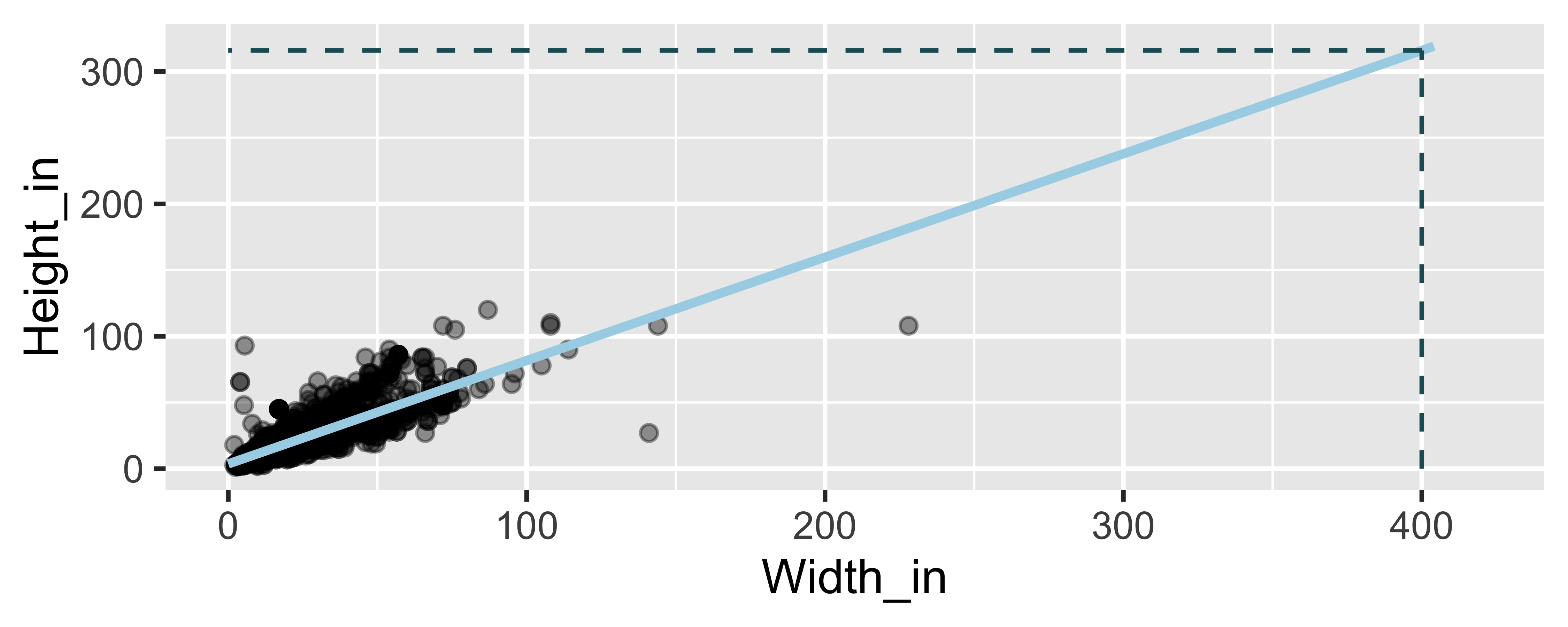
Watch out for extrapolation!

"When those blizzards hit the East Coast this winter, it proved to my satisfaction that global warming was a fraud. That snow was freezing cold. But in an alarming trend, temperatures this spring have risen. Consider this: On February 6th it was 10 degrees. Today it hit almost 80. At this rate, by August it will be 220 degrees. So clearly folks the climate debate rages on."¹
Stephen Colbert, April 6th, 2010

Measuring the strength of the fit

• The strength of the fit of a linear model is most commonly evaluated using $R^2$.
• It tells us what percent of variability in the response variable is explained by the model.
• The remainder of the variability is explained by variables not included in the model.

Height vs. lanscape features

m_ht_lands <- lm(Height_in ~ factor(landsALL), data = pp)
glance(m_ht_lands)$r.squared

## [1] 0.03456724

(a) 3.5% of the variability in heights of painting can be explained by whether or not the painting has landscape features.

(b) 3.5% of the variability in whether a painting has landscape features can be explained by heights of paintings.

(c) This model predicts 3.5% of heights of paintings accurately.

(d) This model predicts 3.5% of whether a painting has landscape features accurately.

(e) 3.5% of the time there is an association between whether a painting has landscape features and its height.

Height vs. width

glance(m_ht_wt)

## # A tibble: 1 x 11
##   r.squared adj.r.squared sigma statistic p.value    df  logLik    AIC
##       <dbl>         <dbl> <dbl>     <dbl>   <dbl> <int>   <dbl>  <dbl>
## 1     0.683         0.683  8.30     6749.       0     2 -11083. 22173.
## # … with 3 more variables: BIC <dbl>, deviance <dbl>, df.residual <int>

glance(m_ht_wt)$r.squared # extract R-squared

## [1] 0.6829468

Roughly 68% of the variability in heights of paintings can be explained by their widths.

Not-so-tidy regression output

• You might come accross these in your googling adventures, but we'll try to stay away from them
• Not because they are wrong, but because they don't result in tidy data frames as results.

Not-so-tidy regression output (1)

Option 1:

m_ht_wt

## 
## Call:
## lm(formula = Height_in ~ Width_in, data = pp)
## 
## Coefficients:
## (Intercept)     Width_in  
##      3.6214       0.7808

Not-so-tidy regression output (2)

Option 2:

summary(m_ht_wt)

## 
## Call:
## lm(formula = Height_in ~ Width_in, data = pp)
## 
## Residuals:
##     Min      1Q  Median      3Q     Max 
## -86.714  -4.384  -2.422   3.169  85.084 
## 
## Coefficients:
##             Estimate Std. Error t value Pr(>|t|)
## (Intercept) 3.621406   0.253860   14.27   <2e-16
## Width_in    0.780796   0.009505   82.15   <2e-16
## 
## Residual standard error: 8.304 on 3133 degrees of freedom
##   (258 observations deleted due to missingness)
## Multiple R-squared:  0.6829,    Adjusted R-squared:  0.6828 
## F-statistic:  6749 on 1 and 3133 DF,  p-value: < 2.2e-16

Review

• Each variable forms a column.
• Each observation forms a row.
• Each type of observational unit forms a table.

Tidy regression output

Achieved with functions from the broom package:

• tidy: Constructs a data frame that summarizes the model's statistical findings: coefficient estimates, standard errors, test statistics, p-values.
• glance: Constructs a concise one-row summary of the model. This typically contains values such as $R^2$, adjusted $R^2$, and residual standard error that are computed once for the entire model.
• augment: Adds columns to the original data that was modeled. This includes predictions and residuals.

We've already seen...

• Tidy your model's statistical findings

tidy(m_ht_wt)

## # A tibble: 2 x 5
##   term        estimate std.error statistic  p.value
##   <chr>          <dbl>     <dbl>     <dbl>    <dbl>
## 1 (Intercept)    3.62    0.254        14.3 8.82e-45
## 2 Width_in       0.781   0.00950      82.1 0.

• Glance to assess model fit

glance(m_ht_wt)

## # A tibble: 1 x 11
##   r.squared adj.r.squared sigma statistic p.value    df  logLik    AIC
##       <dbl>         <dbl> <dbl>     <dbl>   <dbl> <int>   <dbl>  <dbl>
## 1     0.683         0.683  8.30     6749.       0     2 -11083. 22173.
## # … with 3 more variables: BIC <dbl>, deviance <dbl>, df.residual <int>

Augment data with model results

New variables of note (for now):

• .fitted: Predicted value of the response variable
• .resid: Residuals

augment(m_ht_wt) %>%
  slice(1:5)

## # A tibble: 5 x 10
##   .rownames Height_in Width_in .fitted .se.fit .resid    .hat .sigma
##   <chr>         <dbl>    <dbl>   <dbl>   <dbl>  <dbl>   <dbl>  <dbl>
## 1 1                37     29.5    26.7   0.166  10.3  3.99e-4   8.30
## 2 2                18     14      14.6   0.165   3.45 3.96e-4   8.31
## 3 3                13     16      16.1   0.158  -3.11 3.61e-4   8.31
## 4 4                14     18      17.7   0.152  -3.68 3.37e-4   8.31
## 5 5                14     18      17.7   0.152  -3.68 3.37e-4   8.31
## # … with 2 more variables: .cooksd <dbl>, .std.resid <dbl>

Residuals plot

m_ht_wt_aug <- augment(m_ht_wt)
ggplot(m_ht_wt_aug, mapping = aes(x = .fitted, y = .resid)) +
  geom_point(alpha = 0.5) +
  geom_hline(yintercept = 0, color = "gray", lty = 2) +
  labs(x = "Predicted height", y = "Residuals")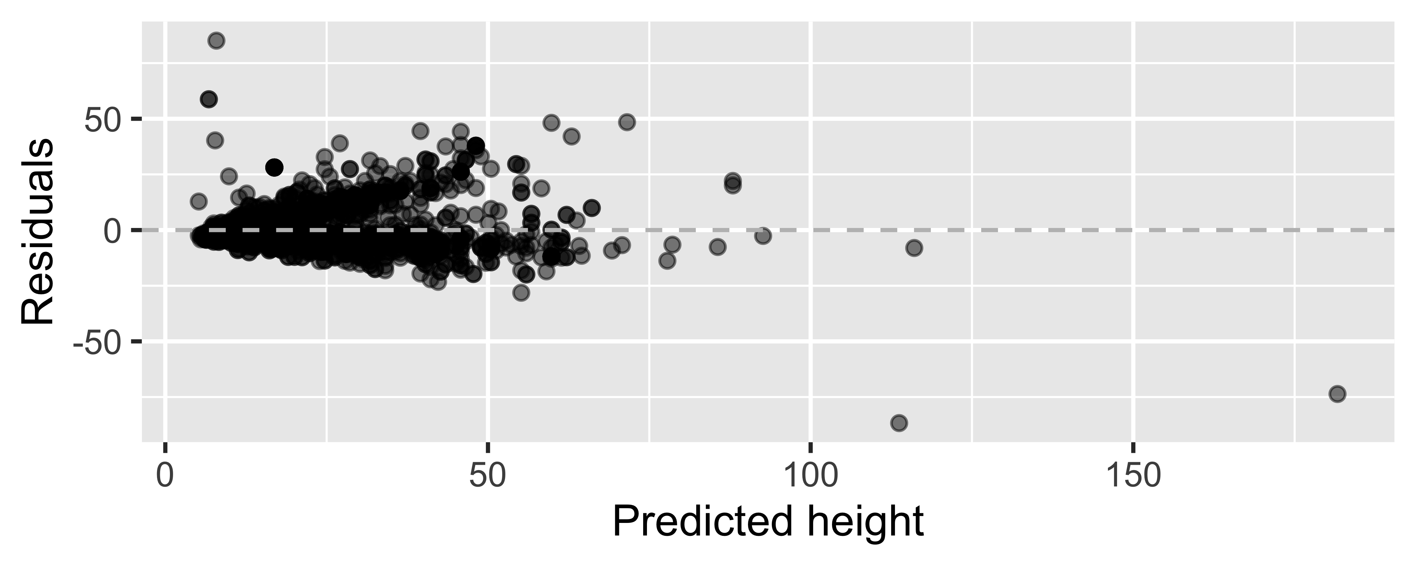

"Linear" models

• We're fitting a "linear" model, which assumes a linear relationship between our explanatory and response variables.
• But how do we assess this?

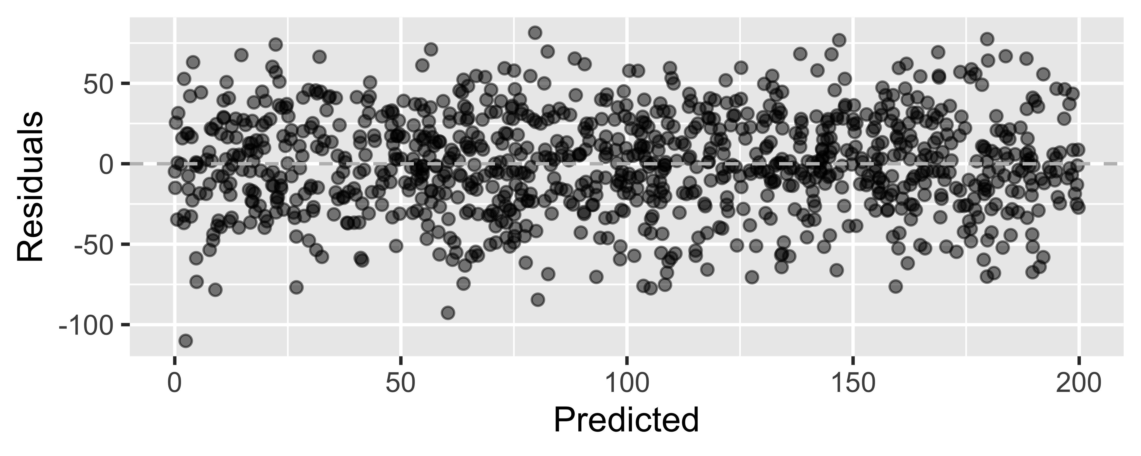
Looking for...

• Residuals distributed randomly around 0
• With no visible pattern along the x or y axes

Not looking for...

Fan shapes

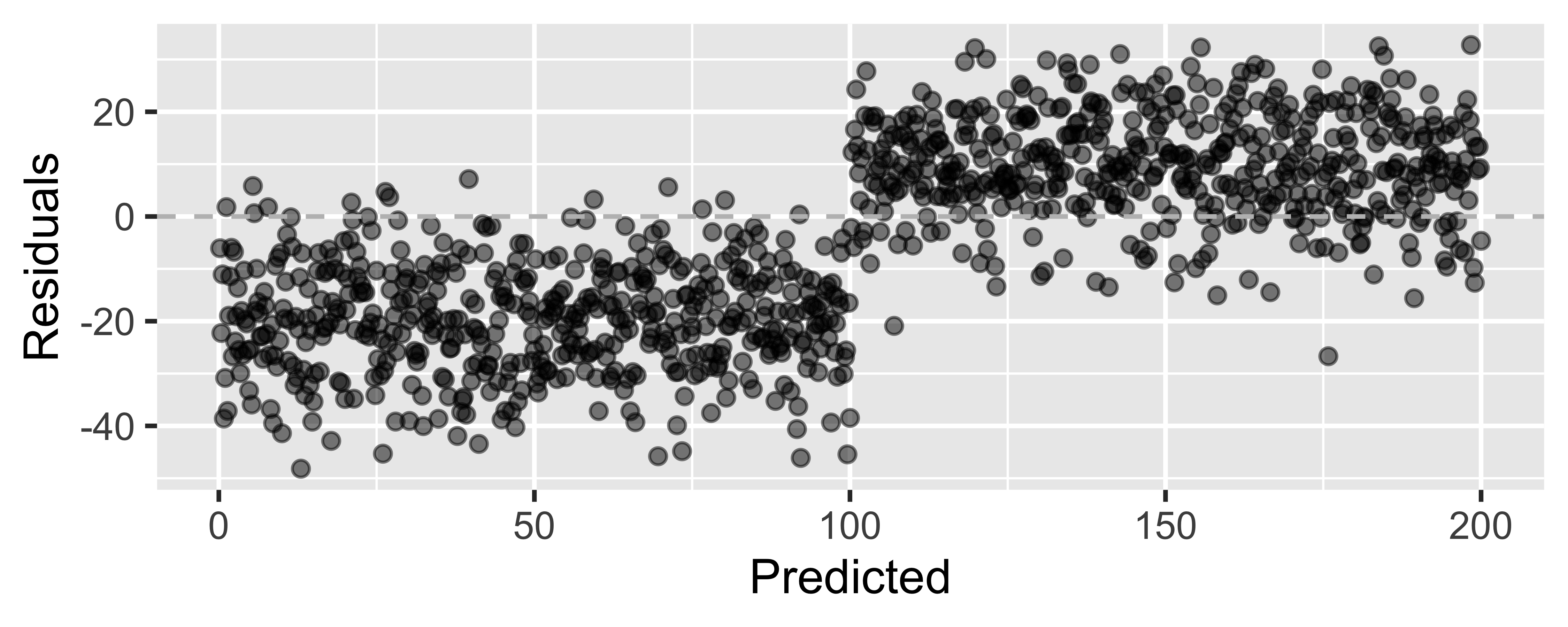
Not looking for...

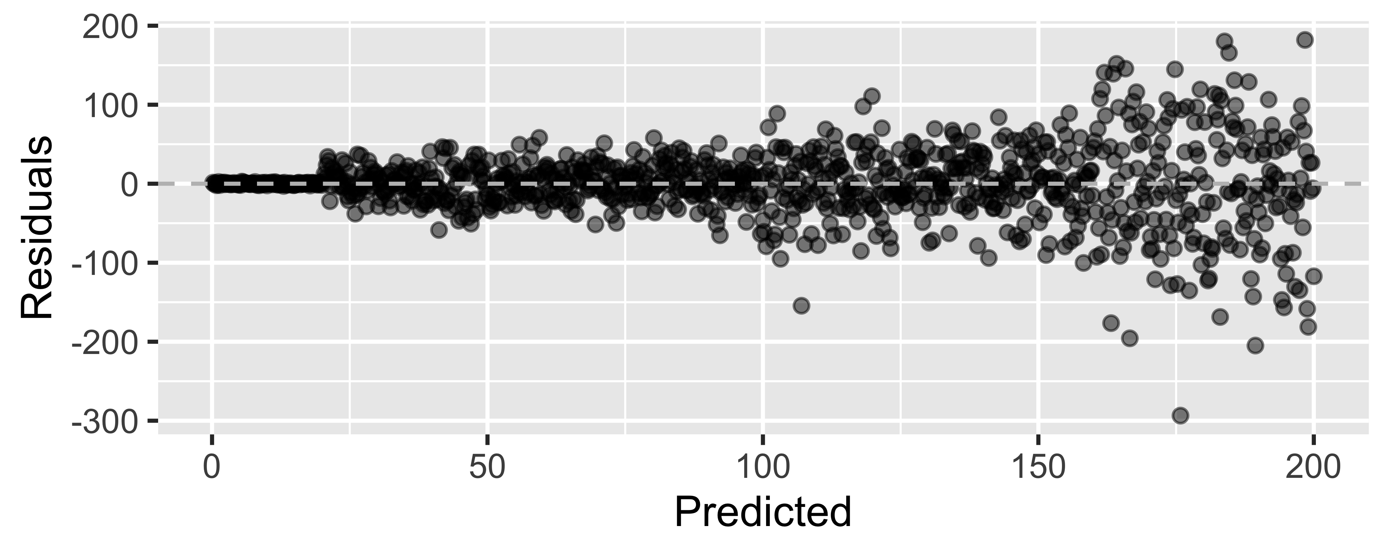
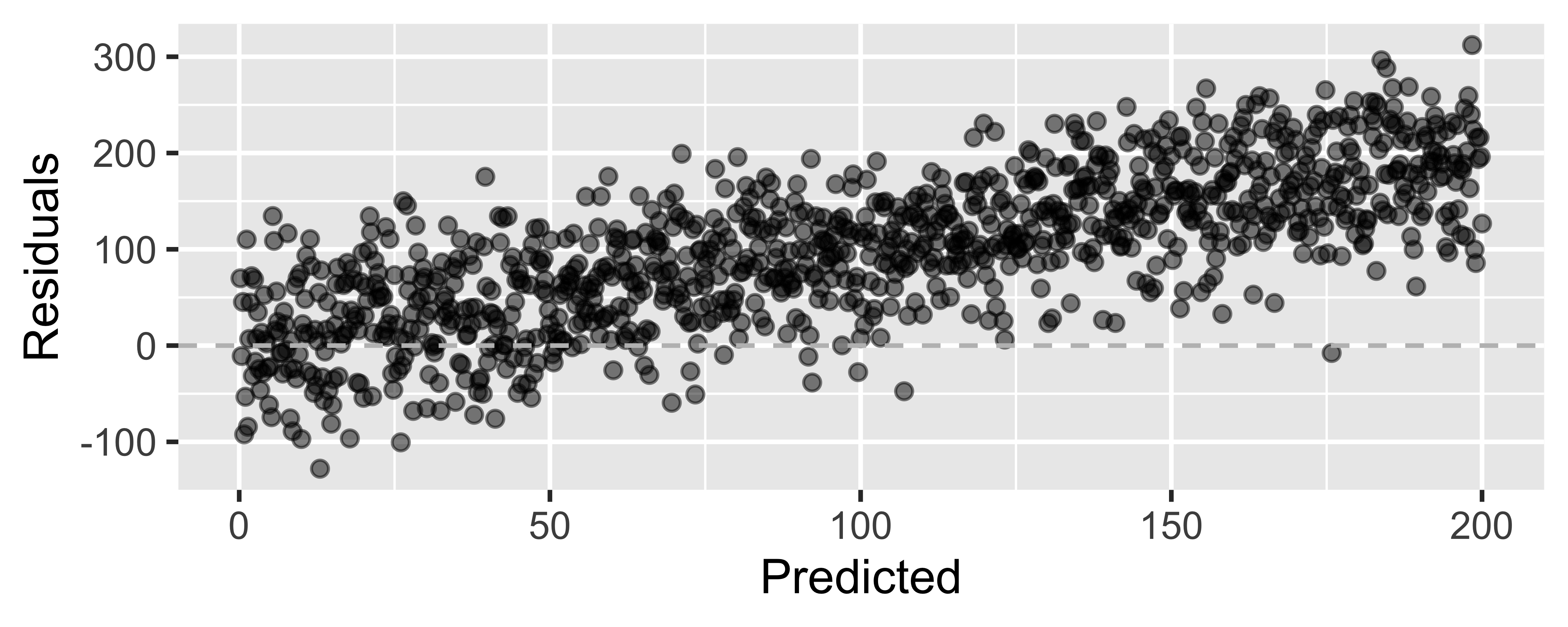
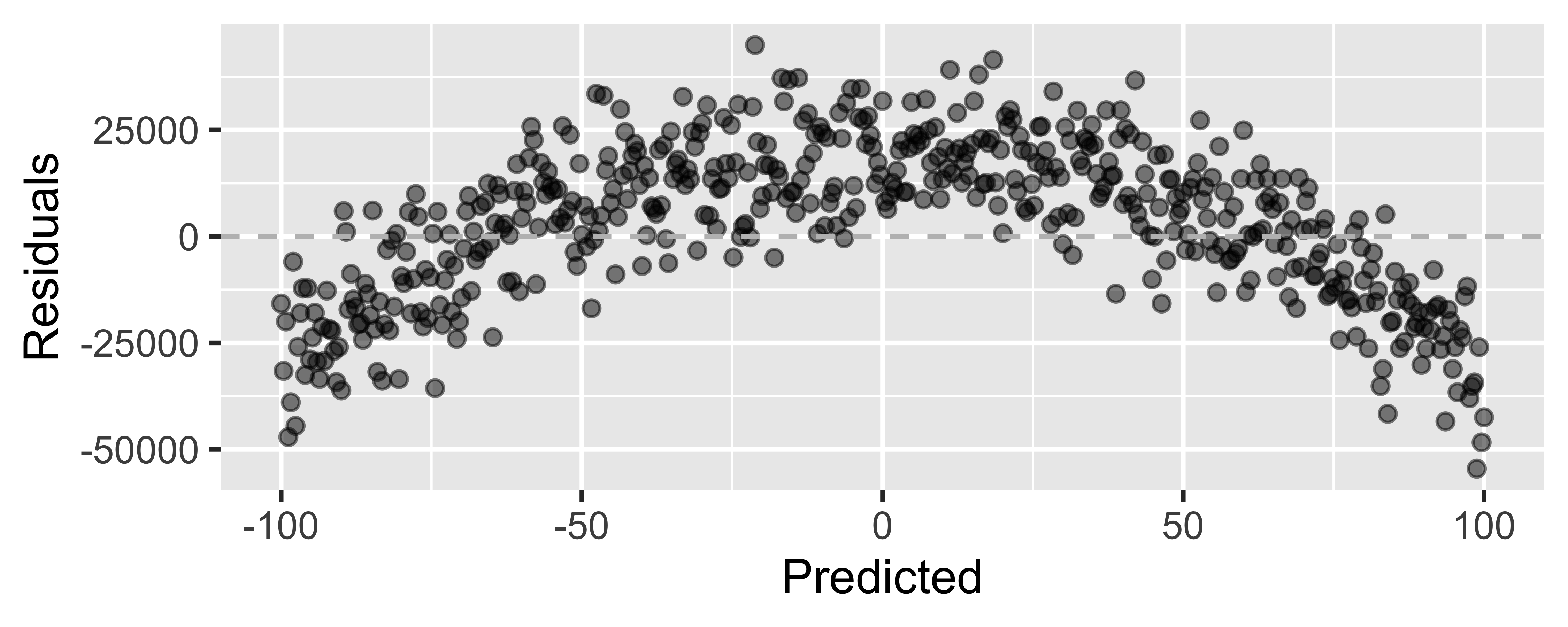
Residuals correlated with predicted values

Not looking for...

Groups of patterns

Not looking for...

Any patterns!